Pierre NICOLAS (1,2) and Florence MURI-MAJOUBE (1)
(1) Laboratoire de Statistique et Génome, CNRS, Tour Évry2, 523 place des terrasses de l'Agora, F-91034 Évry
(2) Laboratoire de Mathématique, Informatique et Génome, INRA, Route de Saint-Cyr, F-78026 Versailles cedex
R'HOM is a set of programs to segment a DNA sequence into a finite number of homogeneous regions. Each region can be composed of several segments. The models used are Hidden Markov Models, HMM (M1-Mk). Segment arrangement is represented by an unobservable first order Markov chain, the hidden state chain (M1). The homogeneous regions are described by different models, more precisely by k-order Markov chains (Mk). Each model has characteristic statistical properties and take into account the local composition in oligonucleotides of length k+1 of the DNA sequence.
Several iterative algorithms are proposed to, on one hand, reconstruct the hidden state chain, that is to identify and locate the homogeneous regions of a given sequence (or a set of sequences), and on the other hand, to estimate the model parameters (state and observation transitions), in order to characterize these regions. When R'HOM is used on a set of sequences, the sequences are assumed to be independently generated using an unique set of parameters for all sequences (leading to a global estimation).
The deterministic EM (Expectation-Maximization) algorithm gives a maximum likelihood estimation. To take into account available information on the model parameters, we also proposed a bayesian estimation with Dirichlet priors (on state and observation transitions) using MCMC (Markov Chain Monte Carlo) methods, more precisely Gibbs sampling. These two iterative procedures, EM and MCMC methods, don't require any learning set of presegmented sequences to give a segmentation of the sequence.
The corresponding programs are:
[1] BIZE, L., MURI, F., SAMSON, F., RODOLPHE, F., EHRLICH, S.D., PRUM,B., BESSIÈRES, P. (1999) ``Searching gene transfers on Bacillus Subtilis using hidden Markov models''. In Recomb'99 Proceedings of the Third Annual International Conference on Computational Molecular Biology.
[2] MURI, F. (1998) ``Modelling bacterial genomes using hidden Markov models''. In Compstat'98 Proceedings in Computational Statistics, (Eds R. Payne and P. Green), pp. 89-100. Heidelberg: Physica-Verlag.
[3] MURI, F.,
CHAUVEAU, D., CELLIER, D. (1998) ``Convergence
Assessment in Latent Variable
Models: ![]() Applications''. In Lecture Notes in Statistics Discretization and
Applications''. In Lecture Notes in Statistics Discretization and ![]() Convergence Assessment (ed C.P.
Robert), Chapter 6, pp. 127-146. Springer-Verlag.
Convergence Assessment (ed C.P.
Robert), Chapter 6, pp. 127-146. Springer-Verlag.
[4] MURI, F. (1997) ``Comparaison d'algorithmes d'identification de
chaînes de Markov cachées et application à la détection de
régions homogènes dans les séquences d'![]() ''.
PhD Thesis,Université Paris V, 1997.
''.
PhD Thesis,Université Paris V, 1997.
[1] CHURCHILL G.A. (1989) ``Stochastic models for heterogeneous DNA sequences''. B. Math. Biol., 51:79-94.
[2] AUDIC S., CLAVERIE JM. (1998) ``Self-identification of protein-coding regions in microbial genomes''. Proc Natl Acad Sci U S A. Aug 18;95(17):10026-31.
[3] L. PESHKIN AND M.S. GELFAND (1999) ``Segmentation of yeast DNA using hidden Markov models''. Bioinformatics, 15:980-986.
[4] OLIVER JL, ROMAN-ROLDAN R, PEREZ J, BERNAOLA-GALVAN P. (1999) SEGMENT: identifying compositional domains in DNA sequences. Bioinformatics. Dec;15(12):974-9.
[5] R.J. BOYS AND D.A. HENDERSON AND D.J. WILKINSON (2000) Detecting homogenous segments in dna sequences by using hidden Markov models. Appl. Stat., 2000, 49, 269-285.
The models used to describe DNA sequence heterogeneities are
Hidden Markov Models (M1-Mk). These models allow to segment a
sequence into a finite number, nstate, regions, that can be
composed of several segments, without any prior knowledge about
their content, size or localization. Segment arrangement
corresponds to an underlying structure of the sequence modelized
by an hidden Markov chain with nstate states, called the
hidden state chain. A DNA sequence is represented by a finite
series
![]() , each letter
, each letter ![]() taken from an alphabet
taken from an alphabet ![]() with nmodal modalities (several type of alphabet are
considered, for instance nmodal=4 letters a,c,g,t,...), and
the corresponding hidden states by a finite series
with nmodal modalities (several type of alphabet are
considered, for instance nmodal=4 letters a,c,g,t,...), and
the corresponding hidden states by a finite series
![]() , each
, each
![]() taking nstate possible values.
taking nstate possible values.
For all the models, the
hidden states are generated according to an homogeneous first
order Markov chain, MC, (M1), with finite state space
![]() , that is the probability of generating a
state at a given position depends only on the previous state.
Moreover, the transition probabilities from a state u to a state
v, denoted by
, that is the probability of generating a
state at a given position depends only on the previous state.
Moreover, the transition probabilities from a state u to a state
v, denoted by
![]() are homogeneous: they don't depend on
the sequence position.
are homogeneous: they don't depend on
the sequence position.
| that we choose as |
 |
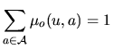
The letters of the sequence, ![]() , appear with a law that depends on
the hidden state
, appear with a law that depends on
the hidden state ![]() . Several models are considered.
. Several models are considered.
 |
 |
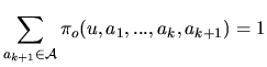
The choice of the order ![]() of the model M1-Mk depends on the
information (local oligonucleotide composition) that ones want to
take into account to characterize the homogeneous regions.
of the model M1-Mk depends on the
information (local oligonucleotide composition) that ones want to
take into account to characterize the homogeneous regions.
For
instance, the M1-M2 model fits on the local trinucleotide
composition of the sequence.
For a given M1-Mk model, rhom.em uses the iterative EM algorithm to reconstruct the hidden state sequence and give an approximation of the maximum likelihood estimator (MLE)
![]() of the model parameters
of the model parameters
![]() .
The
.
The ![]() EM iteration consists in:
EM iteration consists in:
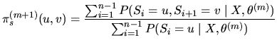
Starting from an initial
value of the model parameters
![]() , E and M steps are alternated until
an iteration
, E and M steps are alternated until
an iteration ![]() for which the difference between the loglikelihood value
for which the difference between the loglikelihood value
![]() of two successive iterations is less than an arbitrary
threshold epsilon. Finaly
of two successive iterations is less than an arbitrary
threshold epsilon. Finaly
![]() and state sequence is reconstructed with the state probabilities
and state sequence is reconstructed with the state probabilities
![]() .
.
Contiguous positions associated to the same
segment class ![]() ,
,
![]() , are
identified as an homogeneous segment of class
, are
identified as an homogeneous segment of class ![]() . All homogeneous
segments of class
. All homogeneous
segments of class ![]() are characterized by the same
are characterized by the same ![]() -nucleotide
composition
-nucleotide
composition
![]() .
.
> rhom.em -model <model_desc> -seq <seq_list> -em <em_param>
> rhom.em -h
The input files contain lists of keywords that must be specified. Comments, always preceded by a "#", can be introduced in the files. A keyword can be followed by a ":", but no space character has to be introduced between the keyword and the ":"
The file ![]() seq_list
seq_list![]() contains the names of the files containing the
sequences to study. The sequences don't have to be in the same
directory, but the corresponding output files are created in the
same directory as the sequence. Each sequence must only contain
the following characters: a, A, c, C, g, G, t, T (ignoring the case). Numeric
characters are ignored.
contains the names of the files containing the
sequences to study. The sequences don't have to be in the same
directory, but the corresponding output files are created in the
same directory as the sequence. Each sequence must only contain
the following characters: a, A, c, C, g, G, t, T (ignoring the case). Numeric
characters are ignored.
sequence1.gb
sequence2.gb
> title
agctgtgt...
Warning the fasta file must contain only one sequence.
title #
agctgtgtaa ...
This file contains the model description with the following keywords:
0: alphabet a, g, c, t (in this order!), nmodal=4
1: alphabet W, S (W=a+t, S=g+c), nmodal=2
2: alphabet R, Y (R=a+g, Y= c+t), nmodal=2
3: amino-acid alphabet, nmodal=20
#M1-M2 with 4 hidden states
model: 2 # M1-M2
type: 0 #alphabet a, g, c, t
nstate: 4 #4 hidden states
This file contains the informations needed to run and initialize EM. The user can give its own initial values for the parameters, or multiple random initializations can be used, followed by likelihood based selection of the best final results. The keywords are:
only when the user specifies its own starting values:
only when multiple random initializations are used:
with specified starting values (for the preceding model description):
#algo EM with 100 iterations. M1-M2 with 4 hidden states. Stopping criteria fixed to 10e-3
niter 100
eps 10e-3

pis #Initial values of state transitions (nstate*nstate=4 * 4)
#state 1 state 2   state 3     state 4
0.948854    0.0502678   0.000877813 1.30941e-28 #state 1
0.0938233   0.896385 1.93881e-57 0.00979151 # state 2
1.4473e-105 1.02748e-93 0.998933 0.00106683 # state 3
0.0308109   2.0568e-06  0.00484188  0.964345 #state 4

mus #Initial values of initial state distribution (1*nstate=1 * 4)
#state 1 state 2   state 3     state 4
0.301835 0.146496 0.496712 0.0551699

pio #Initial values of observation transitions (4*4*4=nstate*nmodal*nmodal)
#state 1
#a       g        c       t
0.250679 0.199376 0.28703 0.262915 # aa
0.262325 0.104503 0.0636073 0.569565 # ag
0.348552 0.0376766 0.356861 0.25691 # ac
0.290229 0.276766 0.253169 0.179837  # at
0.171719 0.263213 0.180284 0.384785  # ga
0.35131 0.421945 0.082876 0.143869  # gg
1.03216e-07 0.227579 0.340905 0.431516 # gc
0.166153 0.428288 0.128137 0.277423 # gt
0.563403 0.148526 0.171301 0.116769 # ca
0.532434 4.38999e-07 0.170677 0.296889  # cg
0.681336 7.41972e-10 0.161307 0.157356  # cc
0.398021 0.117946 0.188856 0.295177  # ct
0.462522 0.250213 0.194246 0.0930196  # ta
0.443759 0.318182 0.139334 0.0987249 # tg
0.722646 0.0339112 0.243443 2.72926e-41 # tc
0.229728 0.227167 0.254991 0.288114 # tt
#state2
0.460708 0.30662 0.216851 0.0158213
...
#state 3
0.225592 0.263064 0.331467 0.179877
...
#state 4
0.312473 0.143202 0.0801305 0.464194
...

muo #Initial values of initial observation distribution
#(4*4=nstate*nmodal)
#state 1
#a       g        c       t
0.12904 0.0747909 0.079439 0.0792296 #a
0.0706479 0.0487123 0.0194636 0.0588641 #g
0.100936 0.00959239 0.0561533 0.0380135 #c
0.0615724 0.0647921 0.0497819 0.0589715 #t
#state2
0.165736 0.0854782 0.0434868 0.0376994
...
#state 3
0.158642 0.0614003 0.0349861 0.0958986
...
#state 4
0.0276459 0.00812737 0.078968 0.0256395
with use of multiple random initialization (for the preceding model description):
#algo EM with 100 iterations. M1-M2 with 4 hidden states.
#Stopping criteria fixed to 10e-3
niter 100
eps 10e-3

pis_sel 0.99
#the diagonal elements of pis are set to 0.99
# Mean length of each region = 100 bp.
niter_sel 100
nb_sel 10
#10 starting points are selected at random for which 100 iterations are made.
#The best path is kept for which niter=100 iterations are made.
The command:
> rhom.em -model <model_desc> -seq <seq_list> -em <em_param>creates the following output files:
The structure of these output files are the same for a random or specified initialization. When a random initialisation is used, two additional files are created:
This file contains informations about the model and algorithm descriptions, initial values of the parameters, successive values of the loglikelihood and the stopping criteria for each iteration, and the final values of the parameters.
hidden state number (nstate): 4
observation modality number (nmodal): 4
maximal iteration number (niter): 100 (working on A,G,C,T)
Markov model order: M1-M2
Algorithm: EM
sequence list file: fic_seq
number of sequences: 2
total sequence length: 8002 sequence files:
    sequence1.gb
    sequence2.gb

#initial values of pis
pis: 0.948854 0.0502678 0.000877813 1.30941e-28 ...

#initial values of mus
mus: 0.301771 0.146465 0.496606 0.0551582

#initial values of pio
pio: 0.250679 0.199376 0.28703 0.262915 0.262325 0.104503...

#initial values of muo
muo: 0.128932 0.0747283 0.0793725 0.0791633 0.0707193...

iteration: 1 loglikelihood: -9833.24
iteration: 2 loglikelihood:-9833.22
diff: 0.0205511

#final values of pis
pis: 0.948683 0.0504397 0.000876873 1.88526e-28 0.0943041 ...

#final values of mus
mus: 0.301963 0.146351 0.496714 0.055186

#final values of pio
pio: 0.250553 0.199383 0.287258 0.262807 0.262736 0.104441 ...

#final values of muo
muo: 0.128992 0.0748365 0.0794692 0.079204 0.0706376 0.0487347 ...


Iteration number: 63 epsilon and loglikelihood diff: 10e-3 0.000205511
R'HOM produces as many .rhom output files as
sequences in the file ![]() seq_list
seq_list![]() . The name of each output file is
sequence_name.rhom. Each file contains a description of the model
and the algorithm parametrization, the state probabilities
. The name of each output file is
sequence_name.rhom. Each file contains a description of the model
and the algorithm parametrization, the state probabilities
![]() estimated with EM, for each position
estimated with EM, for each position ![]() of the
sequence, and all segment class
of the
sequence, and all segment class ![]() , final parameter estimations,
and also characteristic informations of the algorithm.
, final parameter estimations,
and also characteristic informations of the algorithm.
#title and length of the sequence
L43967  #  4001
#type nmodal model nstate algorithm number of self-      number of iter
#                         code      complementary states made
  0    4      2       4     0         0                   2
#type of file (ouptut file of the final results)
0

#estimated state probabilities for all sequence position
#state 1   state 2    state 3   state4
0.00649628 0.00113897  0.991456 0.000908642 # position 1
0.00618641 0.000945452 0.992516 0.000352241 # position 2
0.00586888 0.000870091 0.993261 5.00163e-133 # position 3
...
0.000521638 8.84279e-05 0.997984 0.00140579 # position 4001

# final values of pis
0.948683 0.0504397 0.000876873 1.88526e-28
0.0943041 0.895884 8.89759e-58 0.0098116
1.67912e-106 8.06319e-95 0.998933 0.00106682
0.0308272 1.2522e-06 0.00484352 0.964328

#final values of mus
0.301963 0.146351 0.496714 0.055186

#final values of pio
#state 1
0.250553 0.199383 0.287258 0.262807 0.262736 0.104441 0.0635067...
#state 2
0.461027 0.306671 0.216449 0.0158531 0.12538 0.473632 0.328604...
#state 3
0.46024 0.155891 0.10354 0.280329 0.254131 0.147643 0.163976...
#state 4
7.45071e-51 2.86447e-126 0.576877 0.423123 0.528608 3.81939e-67 ...

#final values of muo
#state 1
0.128992 0.0748365 0.0794692 0.079204 0.0706376 0.0487347 ...
#state 2
0.165878 0.0854007 0.0433873 0.0377102 0.0692985 0.105744 ...
#state 3
0.158642 0.0614002 0.0349862 0.0958989 0.0369068 0.0236469 ...
#state 4
0.0276532 0.00813249 0.0789714 0.025657 0.0157272 0.0166258 ...

#epsilon final value of stopping criteria
10       0.0205511
Remark: this version of R'HOM doesn't consider the possibility of self-complementary states. The number of self-complementary states is set to 0.
Created only for a random initialization.
This file contains the loglikelihood value at the niter_sel iteration for each of the tested nb_sel model (that is for each random starting point), and also specified the selected model.
#nb_sel=10 random starting points are considered for which niter_sel=100 iter are made
#loglikelihood value at the iter niter_sel=100 for the nb_sel=10 tested models.
0 loglikelihood -9851.42
1 loglikelihood -9883.1
2 loglikelihood -9851.94
3 loglikelihood -9879.17
4 loglikelihood -9876.09
5 loglikelihood -9860.59
6 loglikelihood -9894
7 loglikelihood -9897.08
8 loglikelihood -9848.08
9 loglikelihood -9872.34

Best start point used: 8
This file contains the parameter values at the niter_sel iteration for each of the tested nb_sel model (that is for each random starting point). These values can be used as starting points to study local maxima.
#nb_sel=10 random starting points are considered for which niter_sel=100 iter are made
#parameter values at the iter niter_sel=100 for the nb_sel=10 tested models.

pis_sel: 0.99 niter_sel: 100 nb_sel: 10

++++++++++++++++++++++++++++++++
model 0

pis:
0.977557 0.0118793 0.00523414 0.00532981
1.46568e-83 0.994239 0.00190493 0.00385653
0.0006573 0.000402097 0.998941 5.83319e-103
0.00257132 6.11516e-68 8.89454e-50 0.997429

mus:
0.0505506 0.139142 0.497305 0.313215

pio:
1.29304e-135 1.37341e-203 0.376415 0.623585 0.390377 0.405173 ...

muo: 0.0263328 0.0237873 0.0648022 0.0305001 0.032571 0.031781 ...

++++++++++++++++++++++++++++++++
model 1

...

++++++++++++++++++++++++++++++++
model 9

pis:
0.998959 0.000506626 0.000533938 5.87165e-85 ...
mus:
0.5038 0.252605 0.188987 0.0548021
pio:
0.317425 0.230929 0.271109 0.180538 0.217473 0.231578 ...
muo:
0.1288 0.0707994 0.0692565 0.0611432 0.0640931 0.0613545 ...
We thank Annie BOUVIER and Fabrice LEPAGE for their help in R'HOM program developement.
This document was generated using the LaTeX2HTML translator Version 99.2beta8 (1.46)
Copyright © 1993, 1994, 1995, 1996,
Nikos Drakos,
Computer Based Learning Unit, University of Leeds.
Copyright © 1997, 1998, 1999,
Ross Moore,
Mathematics Department, Macquarie University, Sydney.
The command line arguments were:
latex2html -nonavigation -antialias -white -split 0 -notransparent rhom_doc.tex
The translation was initiated by Pierre Nicolas on 2001-10-14